Detection of tree stems with Pyoints
In the following, we try to detect stems in a forest using a three dimensional point cloud generated by a terrestrial laser scanner. The basic steps are:
1. Loading of the point cloud data
2. Calculation of the height above ground
3. Filtering of stem points
4. Identification of stem clusters
5. Fitting of stem vectors
We begin with loading the required modules.
[1]:
import numpy as np

from pyoints import (
    storage,
    Extent,
    filters,
    interpolate,
    clustering,
    classification,
    vector,
)
[2]:
from mpl_toolkits import mplot3d
import matplotlib.pyplot as plt

%matplotlib inline
Loading of the point cloud data
We load a three dimensional point cloud scanned in a forest.
[3]:
lasReader = storage.LasReader('forest.las')
las = lasReader.load()
print(len(las))
482981
We receive a LasRecords instance representing the point cloud. We can treat it like a numpy record array with additional features. So, we inspect its properties first.
[4]:
print('shape:')
print(las.shape)
print('attributes:')
print(las.dtype.descr)
print('projection:')
print(las.proj.proj4)
print('transformation matrix:')
print(np.round(las.t, 2))
print('data:')
print(las)
shape:
(482981,)
attributes:
[('coords', '<f8', (3,)), ('intensity', '|u1'), ('classification', '|u1')]
projection:
+proj=utm +zone=32 +ellps=GRS80 +towgs84=0,0,0,0,0,0,0 +units=m +no_defs
transformation matrix:
[[ 1.00000000e+00  0.00000000e+00  0.00000000e+00  3.64187980e+05]
 [ 0.00000000e+00  1.00000000e+00  0.00000000e+00  5.50957771e+06]
 [ 0.00000000e+00  0.00000000e+00  1.00000000e+00 -1.58000000e+00]
 [ 0.00000000e+00  0.00000000e+00  0.00000000e+00  1.00000000e+00]]
data:
[([ 3.64188062e+05,  5.50957772e+06, -1.28810938e+00], 216, 2)
 ([ 3.64187976e+05,  5.50957776e+06, -1.27100996e+00], 213, 2)
 ([ 3.64188095e+05,  5.50957776e+06, -1.30598884e+00], 214, 2) ...
 ([ 3.64193543e+05,  5.50958151e+06,  1.97219206e+01], 171, 5)
 ([ 3.64193519e+05,  5.50958148e+06,  1.97416807e+01], 160, 5)
 ([ 3.64193506e+05,  5.50958148e+06,  1.97642104e+01], 168, 5)]
Calculation of the height above ground
The LAS file provides some altitude values. But, we are interested in the height above ground instead. So, we select points representing the ground first, to fit a Digital Elevation Model (DEM). Using the DEM we calculate the height above ground for each point.
We use a DEM filter with a resolution of 0.5m. The filter selects local minima and guarantees a horizontal point distance of at least 0.5m and an altitude change between neighbored points below 50 degree.
[5]:
grd_ids = filters.dem_filter(las.coords, 0.5, max_angle=50)
print(grd_ids)
[ 97192  91536  96140  39010  94076  16662  10183 104165  85384  86854
 102761  38482  83712 102151 116834 105635 101280 118048 124970  87311
 108306  40907 123517 114405  13055 112076  24044  36647  51692  12269
  37402 256997 252300 266541  44324 109408  25316 265679 256605  32073
  45612 258610 252564 255461  42903 187875  27079  20457   6038 268661
 122507 271648  31654 167342 275851 260214 262363 189776 183189 276683
   5855 262318 261194 182891 278869  28162 162688 191363 290879 309455
 277489 272069 285002 196335 287382 283646 174355 319378 290570 312708
 165914 170659 192385 308441 199039 179555 314480 298770 195052 200959
 194685 220857 317956 212307 312093 211194 201875 203803 300082]
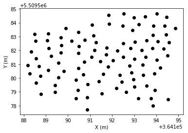
We have received a list of point indices which is used to select the desired representative ground points. So, we update the classification field for these points and plot them.
[6]:
las.classification[grd_ids] = 22
[7]:
plt.scatter(*las[las.classification == 22].coords[:, :2].T, color='black')
plt.xlabel('X (m)')
plt.ylabel('Y (m)')
plt.show()
Now, we fit a DEM using a nearest neighbor interpolator.
[8]:
xy = las.coords[grd_ids, :2]
z = las.coords[grd_ids, 2]
dem = interpolate.KnnInterpolator(xy, z)
Finally, we calculate the height above ground and add a corresponding attribute to the point cloud.
[9]:
height = las.coords[:, 2] - dem(las.coords)
las = las.add_fields([('height', float)], data=[height])
print(las.dtype.descr)
[('coords', '<f8', (3,)), ('intensity', '|u1'), ('classification', '|u1'), ('height', '<f8')]
Filtering of stem points
Now, we try to filter the points subsequently until only points associated with stems remain.
We will focus on points with height above ground greater 0.5m only.
[10]:
fids = np.where(las.height > 0.5)[0]
print(len(fids))
251047
Due to the unnecessary high point density we filter the point cloud using a duplicate point filter. Only a subset of points with a point distance of at least 0.1m is kept.
[11]:
filter_gen = filters.ball(las[fids].indexKD(), 0.1)
fids = fids[list(filter_gen)]
print(len(fids))
12950
Let’s take a look at the remaining point cloud. To receive a nice plot, we define the axis limits first.
[12]:
axes_lims = Extent([
    las.extent().center - 0.5 * las.extent().ranges.max(),
    las.extent().center + 0.5 * las.extent().ranges.max()
])
[13]:
fig = plt.figure(figsize=(15, 15))
ax = plt.axes(projection='3d')
ax.set_xlim(axes_lims[0], axes_lims[3])
ax.set_ylim(axes_lims[1], axes_lims[4])
ax.set_zlim(axes_lims[2], axes_lims[5])
ax.set_xlabel('X (m)')
ax.set_ylabel('Y (m)')
ax.set_zlabel('Z (m)')

ax.plot_trisurf(*las[las.classification == 22].coords.T, cmap='gist_earth')
ax.scatter(*las[fids].coords.T, c=las.height[fids], cmap='coolwarm', marker='.')
plt.show()
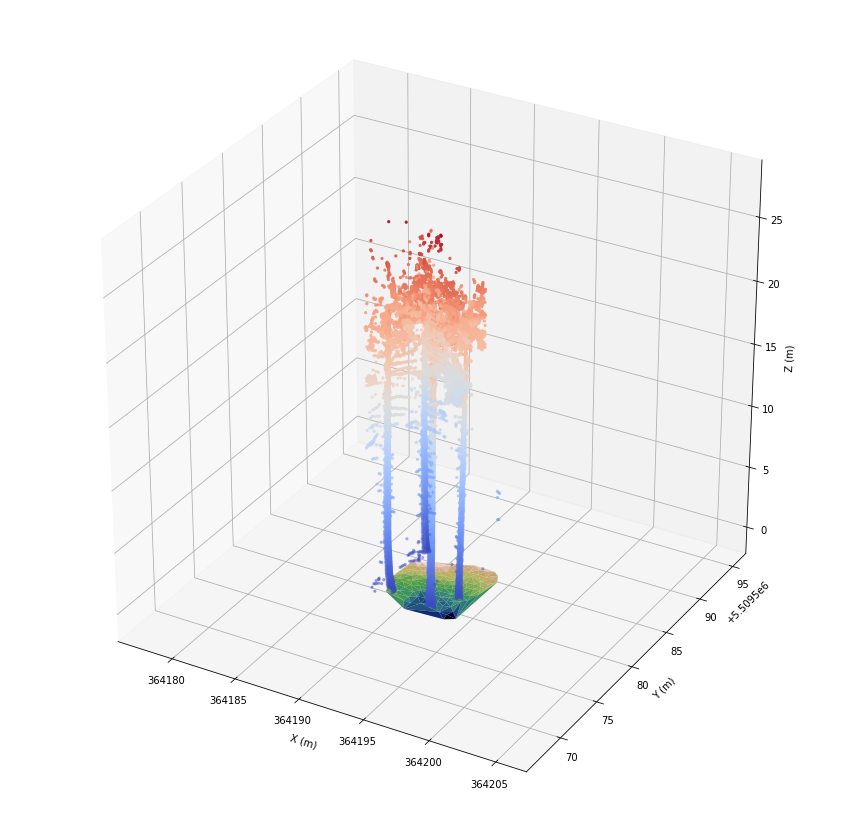
We can see four trees with linear stems. But, there are a lot of points associated with branches or leaves. We assign class 23 to the selected points for later visualization.
[14]:
las.classification[fids] = 23
To reduce noise, we only keep points with a lot of neighbors.
[15]:
count = las[fids].indexKD().ball_count(0.3)
fids = fids[count > 10]
print(len(fids))
las.classification[fids] = 24
10132
[16]:
fig = plt.figure(figsize=(15, 15))
ax = plt.axes(projection='3d')
ax.set_xlim(axes_lims[0], axes_lims[3])
ax.set_ylim(axes_lims[1], axes_lims[4])
ax.set_zlim(axes_lims[2], axes_lims[5])
ax.set_xlabel('X (m)')
ax.set_ylabel('Y (m)')
ax.set_zlabel('Z (m)')

ax.plot_trisurf(*las[las.classification == 22].coords.T, cmap='gist_earth')
ax.scatter(*las[las.classification == 23].coords.T, color='gray', marker='.')
ax.scatter(*las[las.classification == 24].coords.T, color='red', marker='.')
plt.show()
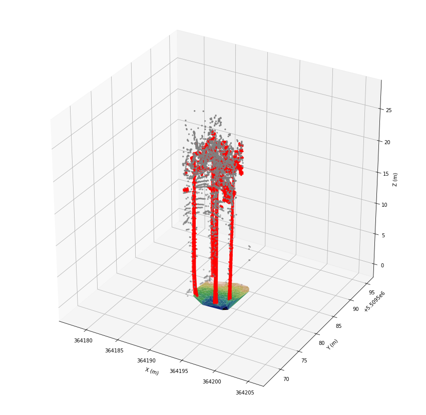
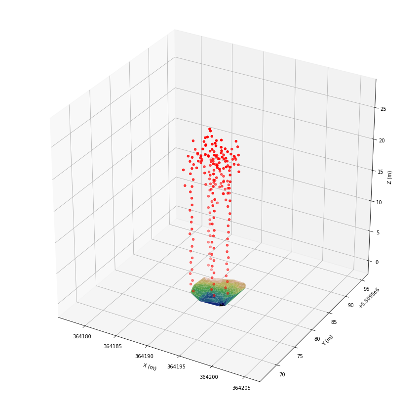
That’s much better, but we are interested in the linear shape of the stems only. So, we filter with a radius of 1 m to remove similar points. This results in a point cloud with point distances of at least 1 m.
[17]:
filter_gen = filters.ball(las[fids].indexKD(), 1.0)
fids = fids[list(filter_gen)]
print(len(fids))
las.classification[fids] = 25
193
[18]:
fig = plt.figure(figsize=(15, 15))
ax = plt.axes(projection='3d')
ax.set_xlim(axes_lims[0], axes_lims[3])
ax.set_ylim(axes_lims[1], axes_lims[4])
ax.set_zlim(axes_lims[2], axes_lims[5])
ax.set_xlabel('X (m)')
ax.set_ylabel('Y (m)')
ax.set_zlabel('Z (m)')

ax.plot_trisurf(*las[las.classification == 22].coords.T, cmap='gist_earth')
ax.scatter(*las[las.classification == 25].coords.T, color='red')
plt.show()
For dense point clouds, the filtering technique would result in point distances in a range of 1m to 2m. Thus, we can assume that linear arranged points should have 2 to 3 neighboring points within a radius of 1.5 m.
[19]:
count = las[fids].indexKD().ball_count(1.5)
fids = fids[np.all((count >= 2, count <= 3), axis=0)]
print(len(fids))
las.classification[fids] = 26
88
[20]:
fig = plt.figure(figsize=(15, 15))
ax = plt.axes(projection='3d')
ax.set_xlim(axes_lims[0], axes_lims[3])
ax.set_ylim(axes_lims[1], axes_lims[4])
ax.set_zlim(axes_lims[2], axes_lims[5])
ax.set_xlabel('X (m)')
ax.set_ylabel('Y (m)')
ax.set_zlabel('Z (m)')

ax.plot_trisurf(*las[las.classification == 22].coords.T, cmap='gist_earth')
ax.scatter(*las[las.classification == 25].coords.T, color='gray', marker='.')
ax.scatter(*las[las.classification == 26].coords.T, color='red')
plt.show()
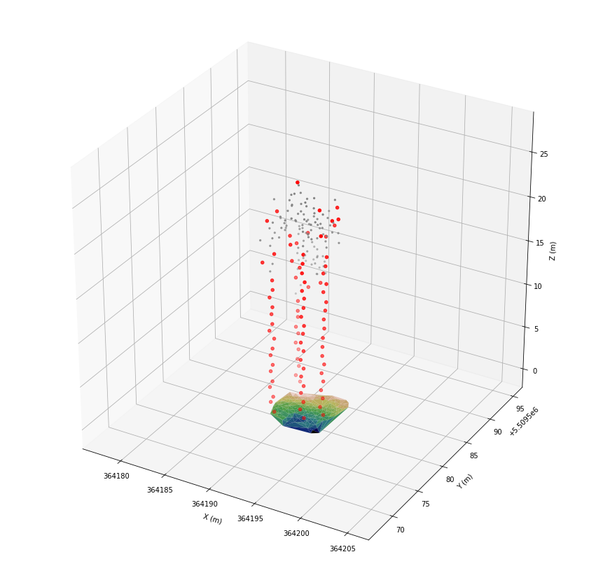
After applying the filters the stems are clearly visible. Thus, we can proceed with the actual detection of the stems.
Identification of stem clusters
We can detect the stems easily by clustering the previously filtered points. For this purpose we apply the DBSCAN algorithm.
[21]:
cluster_indices = clustering.dbscan(las[fids].indexKD(), 2, epsilon=1.5)
print('number of points:')
print(len(cluster_indices))
print('cluster IDs:')
print(np.unique(cluster_indices))
number of points:
88
cluster IDs:
[-1  0  1  2  3  4  5  6]
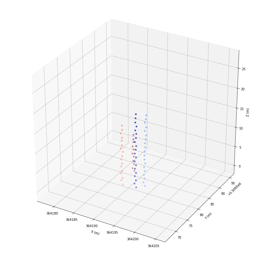
In the next step, we remove small clusters and unassigned points. In addition, we add an additional field, providing the tree ID.
[22]:
cluster_dict = classification.classes_to_dict(cluster_indices, ids=fids, min_size=5)
cluster_indices = classification.dict_to_classes(cluster_dict, len(las))
print('tree IDs:')
print(cluster_dict.keys())
print('cluster_dict:')
print(cluster_dict)
tree IDs:
dict_keys([2, 3, 5, 6])
cluster_dict:
{2: [371973, 371173, 369487, 368857, 366101, 365936, 160689, 159509, 156897, 155653, 152232, 148925, 147360, 144290, 142432, 139379, 137708, 133495, 131557, 90638], 3: [374660, 370651, 370361, 367940, 367297, 162020, 161457, 158619, 154987, 154022, 150829, 150016, 146010, 144831, 141239, 139771, 135805, 133929, 129305], 5: [335645, 77637, 76803, 74807, 73937, 71618, 69644, 69372, 67774, 65755, 63816, 62705, 60297, 59194, 56386, 54681, 19293], 6: [243995, 242571, 241219, 239584, 238103, 235757, 234354, 232652, 231017, 229229, 209774]}
[23]:
las = las.add_fields([('tree_id', int)])
las.tree_id[:] = -1
for tree_id in cluster_dict:
    las.tree_id[cluster_dict[tree_id]] = tree_id
[24]:
fig = plt.figure(figsize=(15, 15))
ax = plt.axes(projection='3d')
ax.set_xlim(axes_lims[0], axes_lims[3])
ax.set_ylim(axes_lims[1], axes_lims[4])
ax.set_zlim(axes_lims[2], axes_lims[5])
ax.set_xlabel('X (m)')
ax.set_ylabel('Y (m)')
ax.set_zlabel('Z (m)')

ax.scatter(*las[las.tree_id > -1].coords.T, c=las.tree_id[las.tree_id > -1], cmap='coolwarm')
plt.show()
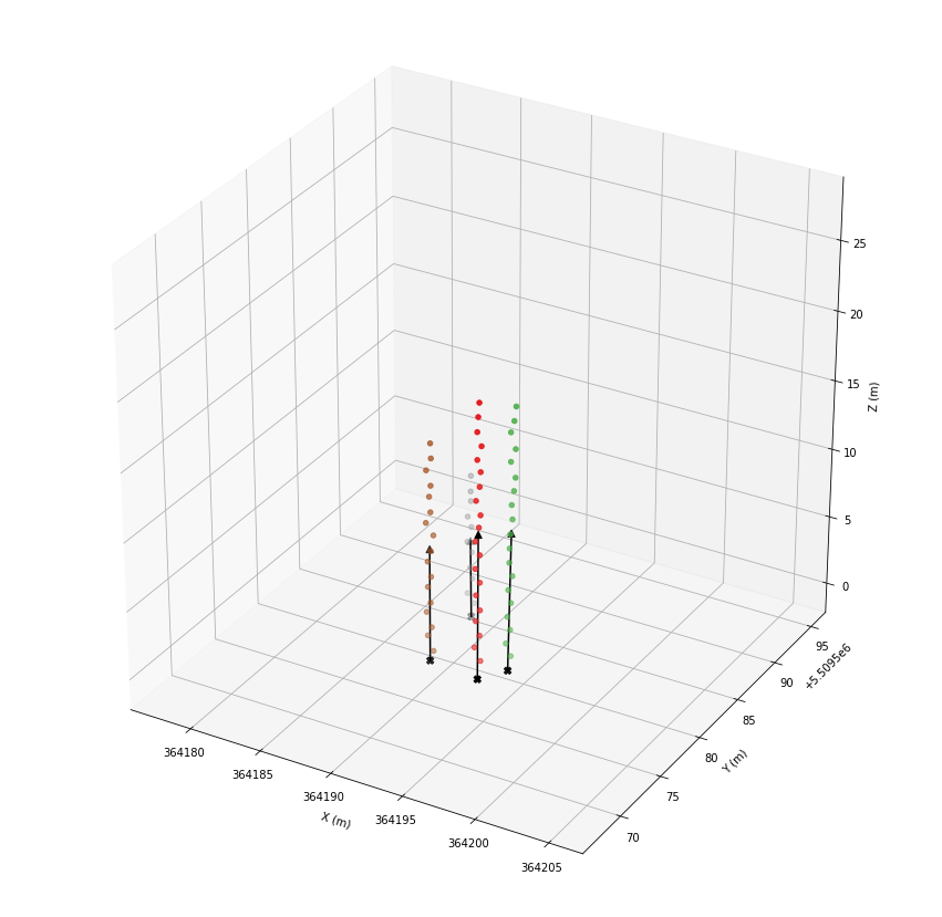
Fitting of stem vectors
To model the stems, we it a vector to each stem.
[25]:
stems = {
    tree_id: vector.Vector.from_coords(las[idx].coords)
    for tree_id, idx in cluster_dict.items()
}
Finally, we determinate the tree root coordinates of the stems by calculating the intersection points with the surface.
[26]:
roots = {
    tree_id: vector.vector_surface_intersection(stem, dem)
    for tree_id, stem in stems.items()
}
origins = { tree_id: stem.origin for tree_id, stem in stems.items()}
[27]:
fig = plt.figure(figsize=(15, 15))
ax = plt.axes(projection='3d')
ax.set_xlim(axes_lims[0], axes_lims[3])
ax.set_ylim(axes_lims[1], axes_lims[4])
ax.set_zlim(axes_lims[2], axes_lims[5])
ax.set_xlabel('X (m)')
ax.set_ylabel('Y (m)')
ax.set_zlabel('Z (m)')

ax.scatter(*las[las.tree_id > -1].coords.T, c=las.tree_id[las.tree_id > -1], cmap='Set1')
ax.scatter(*zip(*roots.values()), color='black', marker='X', s=40)
ax.scatter(*zip(*origins.values()), color='black', cmap='Set1', marker='^', s=40)
for tree_id in roots.keys():
    coords = np.vstack([roots[tree_id], origins[tree_id]])
    ax.plot(*coords.T, color='black')
plt.show()