Getting started
In this tutorial we will learn the basics of raster and point cloud processing using Pyoints.
We begin with loading the required modules.
[1]:
import numpy as np

from pyoints import (
    nptools,
    Proj,
    GeoRecords,
    Grid,
    Extent,
    transformation,
    filters,
    clustering,
    classification,
    smoothing,
)
[2]:
from mpl_toolkits import mplot3d
import matplotlib.pyplot as plt

%matplotlib inline
Grid
We create a two dimensional raster by providing a projection system, a transformation matrix and some data. The transformation matrix defines the origin and scale of the raster. For this example, we just use the default projection system.
[3]:
print('projection')
proj = Proj()
print(proj)

print('numpy record array:')
rec = nptools.recarray(
    {'indices': np.mgrid[0:50, 0:30].T},
    dim=2
)
print(rec.shape)
print(rec.dtype.descr)

print('transformation matrix')
T = transformation.matrix(t=[-15, 10], s=[0.8, -0.8])
print(T)
projection
proj4: +proj=latlong +datum=WGS84 +to +proj=latlong +datum=WGS84 +units=m +no_defs
numpy record array:
(30, 50)
[('indices', '<i8', (2,))]
transformation matrix
[[  0.8   0.  -15. ]
 [  0.   -0.8  10. ]
 [  0.    0.    1. ]]
[4]:
grid = Grid(proj, rec, T)
Let’s inspect the properties of the raster.
[5]:
print('shape:')
print(grid.shape)
print('number of cells:')
print(grid.count)
print('fields:')
print(grid.dtype)
print('projection:')
print(grid.proj)
print('transformation matrix:')
print(np.round(grid.t, 2))
print('origin:')
print(np.round(grid.t.origin, 2).tolist())
print('extent:')
print(np.round(grid.extent(), 2).tolist())
shape:
(30, 50)
number of cells:
1500
fields:
(numpy.record, [('indices', '<i8', (2,)), ('coords', '<f8', (2,))])
projection:
proj4: +proj=latlong +datum=WGS84 +to +proj=latlong +datum=WGS84 +units=m +no_defs
transformation matrix:
[[  0.8   0.  -15. ]
 [  0.   -0.8  10. ]
 [  0.    0.    1. ]]
origin:
[-15.0, 10.0]
extent:
[-14.6, -13.6, 24.6, 9.6]
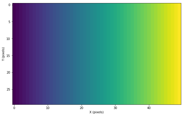
Now, we visualize the x ‘indices’ of the raster.
[6]:
fig = plt.figure(figsize=(10, 10))
plt.xlabel('X (pixels)')
plt.ylabel('Y (pixels)')

plt.imshow(grid.indices[:, :, 0])
plt.show()
You might have noticed, that the field ‘coords’ has been implicitly added to the record array. The coordinates correspond to the centers of the raster cells.
[7]:
print(np.round(grid.coords, 2))
[[[-14.6   9.6]
  [-13.8   9.6]
  [-13.    9.6]
  ...
  [ 23.    9.6]
  [ 23.8   9.6]
  [ 24.6   9.6]]

 [[-14.6   8.8]
  [-13.8   8.8]
  [-13.    8.8]
  ...
  [ 23.    8.8]
  [ 23.8   8.8]
  [ 24.6   8.8]]

 [[-14.6   8. ]
  [-13.8   8. ]
  [-13.    8. ]
  ...
  [ 23.    8. ]
  [ 23.8   8. ]
  [ 24.6   8. ]]

 ...

 [[-14.6 -12. ]
  [-13.8 -12. ]
  [-13.  -12. ]
  ...
  [ 23.  -12. ]
  [ 23.8 -12. ]
  [ 24.6 -12. ]]

 [[-14.6 -12.8]
  [-13.8 -12.8]
  [-13.  -12.8]
  ...
  [ 23.  -12.8]
  [ 23.8 -12.8]
  [ 24.6 -12.8]]

 [[-14.6 -13.6]
  [-13.8 -13.6]
  [-13.  -13.6]
  ...
  [ 23.  -13.6]
  [ 23.8 -13.6]
  [ 24.6 -13.6]]]
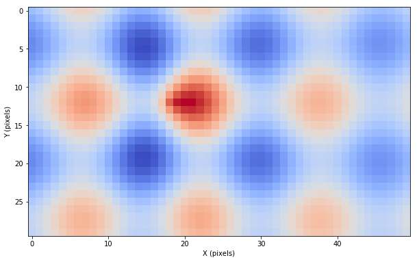
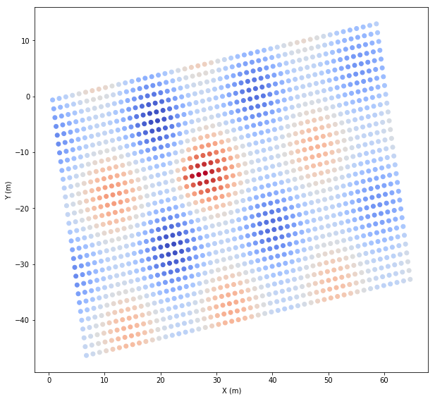
Based on these coordinates we create an additional field representing a surface.
[8]:
x = grid.coords[:, :, 0]
y = grid.coords[:, :, 1]
dist = np.sqrt(x ** 2 + y ** 2)
z = 9 + 10 * (np.sin(0.5 * x) / np.sqrt(dist + 1) + np.cos(0.5 * y) / np.sqrt(dist + 1))
grid = grid.add_fields([('z', float)], data=[z])
print(grid.dtype.descr)
[('indices', '<i8', (2,)), ('coords', '<f8', (2,)), ('z', '<f8')]
[9]:
fig = plt.figure(figsize=(10, 10))
plt.xlabel('X (pixels)')
plt.ylabel('Y (pixels)')

plt.imshow(grid.z, cmap='coolwarm')
plt.show()
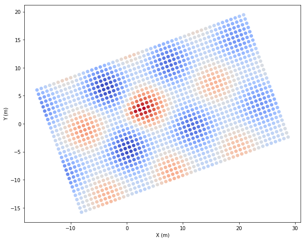
If we like to treat the raster as a point cloud or list of points, we call the ‘records’ function. As a result we receive a flattened version of the raster records.
[10]:
print('records type:')
print(type(grid.records()))
print('records shape:')
print(grid.records().shape)
print('coords:')
print(np.round(grid.records().coords, 2))
records type:
<class 'pyoints.grid.grid.Grid'>
records shape:
(1500,)
coords:
[[-14.6   9.6]
 [-13.8   9.6]
 [-13.    9.6]
 ...
 [ 23.  -13.6]
 [ 23.8 -13.6]
 [ 24.6 -13.6]]
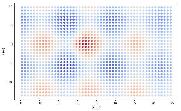
We use these flattened coordinates to visualize the centers of the raster cells.
[11]:
fig = plt.figure(figsize=(10, 10))
ax = plt.axes(aspect='equal')
plt.xlabel('X (m)')
plt.ylabel('Y (m)')

plt.scatter(*grid.records().coords.T, c=grid.records().z, cmap='coolwarm')
plt.show()
GeoRecords
The ‘Grid’ class presented before extends the ‘GeoRecords’ class. Grid objects, like rasters or voxels are well structured, while GeoRecords in general are just a collection of points.
To understand the usage of the GeoRecords, we crate a three dimensional point cloud using the coordinates derived before. We also use the same coordinate reference system. The creation of a GeoRecord array requires for a record array with at least a field ‘coords’ specifying the point coordinates.
[12]:
rec = nptools.recarray({
    'coords': np.vstack([
            grid.records().coords[:, 0],
            grid.records().coords[:, 1],
            grid.records().z
    ]).T,
    'z': grid.records().z
})
geoRecords = GeoRecords(grid.proj, rec)
We inspect the properties of the point cloud first.
[13]:
print('shape:')
print(geoRecords.shape)
print('number of points:')
print(geoRecords.count)
print('fields:')
print(geoRecords.dtype)
print('projection:')
print(geoRecords.proj)
print('transformation matrix:')
print(np.round(geoRecords.t, 2))
print('origin:')
print(np.round(geoRecords.t.origin, 2).tolist())
print('extent:')
print(np.round(geoRecords.extent(), 2).tolist())
shape:
(1500,)
number of points:
1500
fields:
(numpy.record, [('coords', '<f8', (3,)), ('z', '<f8')])
projection:
proj4: +proj=latlong +datum=WGS84 +to +proj=latlong +datum=WGS84 +units=m +no_defs
transformation matrix:
[[  1.     0.     0.   -14.6 ]
 [  0.     1.     0.   -13.6 ]
 [  0.     0.     1.     1.88]
 [  0.     0.     0.     1.  ]]
origin:
[-14.6, -13.6, 1.88]
extent:
[-14.6, -13.6, 1.88, 24.6, 9.6, 19.61]
Before we visualize the point cloud, we define the axis limits.
[14]:
axes_lims = Extent([
    geoRecords.extent().center - 0.5 * geoRecords.extent().ranges.max(),
    geoRecords.extent().center + 0.5 * geoRecords.extent().ranges.max()
])
[15]:
fig = plt.figure(figsize=(15, 15))
ax = plt.axes(projection='3d')
ax.set_xlim(axes_lims[0], axes_lims[3])
ax.set_ylim(axes_lims[1], axes_lims[4])
ax.set_zlim(axes_lims[2], axes_lims[5])
ax.set_xlabel('X (m)')
ax.set_ylabel('Y (m)')
ax.set_zlabel('Z (m)')

ax.scatter(*geoRecords.coords.T, c=geoRecords.z, cmap='coolwarm')
plt.show()

Transformation
For some applications we might like to transform the raster coordinates a bit.
[16]:
T = transformation.matrix(t=[15, -10], s=[1.5, 2], r=10*np.pi/180, order='trs')
tcoords = transformation.transform(grid.records().coords, T)
[17]:
fig = plt.figure(figsize=(10, 10))
ax = plt.axes(aspect='equal')
plt.xlabel('X (m)')
plt.ylabel('Y (m)')

plt.scatter(*tcoords.T, c=grid.records().z, cmap='coolwarm')
plt.show()
Or we roto-translate the raster.
[18]:
T = transformation.matrix(t=[1, 2], r=20*np.pi/180)
grid.transform(T)
[18]:
rec.array([[([ 0,  0], [-16.00290564,   6.02755507],  7.22492983),
            ([ 1,  0], [-15.25115154,   6.30117118],  7.83670869),
            ([ 2,  0], [-14.49939745,   6.5747873 ],  8.69192399), ...,
            ([47,  0], [ 19.3295369 ,  18.88751246],  7.45240576),
            ([48,  0], [ 20.081291  ,  19.16112857],  7.97235695),
            ([49,  0], [ 20.8330451 ,  19.43474469],  8.66432148)],
           [([ 0,  1], [-15.72928952,   5.27580097],  6.27466643),
            ([ 1,  1], [-14.97753543,   5.54941709],  6.87450858),
            ([ 2,  1], [-14.22578133,   5.8230332 ],  7.72147395), ...,
            ([47,  1], [ 19.60315302,  18.13575836],  6.66350211),
            ([48,  1], [ 20.35490711,  18.40937447],  7.19794589),
            ([49,  1], [ 21.10666121,  18.68299059],  7.9045134 )],
           [([ 0,  2], [-15.45567341,   4.52404687],  5.41968082),
            ([ 1,  2], [-14.70391931,   4.79766299],  6.00745844),
            ([ 2,  2], [-13.95216522,   5.0712791 ],  6.84581285), ...,
            ([47,  2], [ 19.87676913,  17.38400426],  5.96308888),
            ([48,  2], [ 20.62852323,  17.65762038],  6.51102379),
            ([49,  2], [ 21.38027732,  17.93123649],  7.23114746)],
           ...,
           [([ 0, 27], [ -8.61527054, -14.26980554],  9.24599585),
            ([ 1, 27], [ -7.86351645, -13.99618943],  9.86919387),
            ([ 2, 27], [ -7.11176235, -13.72257331], 10.72329632), ...,
            ([47, 27], [ 26.717172  ,  -1.40984815],  9.16321474),
            ([48, 27], [ 27.46892609,  -1.13623204],  9.65041211),
            ([49, 27], [ 28.22068019,  -0.86261592], 10.3084549 )],
           [([ 0, 28], [ -8.34165443, -15.02155964],  9.3159224 ),
            ([ 1, 28], [ -7.58990033, -14.74794352],  9.93154535),
            ([ 2, 28], [ -6.83814624, -14.47432741], 10.77365546), ...,
            ([47, 28], [ 26.99078811,  -2.16160225],  9.22523827),
            ([48, 28], [ 27.74254221,  -1.88798613],  9.70847404),
            ([49, 28], [ 28.49429631,  -1.61437002], 10.36182324)],
           [([ 0, 29], [ -8.06803831, -15.77331374],  9.04142244),
            ([ 1, 29], [ -7.31628422, -15.49969762],  9.64458249),
            ([ 2, 29], [ -6.56453012, -15.22608151], 10.46986629), ...,
            ([47, 29], [ 27.26440423,  -2.91335635],  8.98850008),
            ([48, 29], [ 28.01615832,  -2.63974023],  9.47138481),
            ([49, 29], [ 28.76791242,  -2.36612412], 10.12351058)]],
          dtype=[('indices', '<i8', (2,)), ('coords', '<f8', (2,)), ('z', '<f8')])
[19]:
fig = plt.figure(figsize=(10, 10))
ax = plt.axes(aspect='equal')
plt.xlabel('X (m)')
plt.ylabel('Y (m)')

plt.scatter(*grid.records().coords.T, c=grid.records().z, cmap='coolwarm')
plt.show()
IndexKD
The ‘GeoRecords’ class provides a ‘IndexKD’ instance to perform spatial neighborhood queries efficiently.
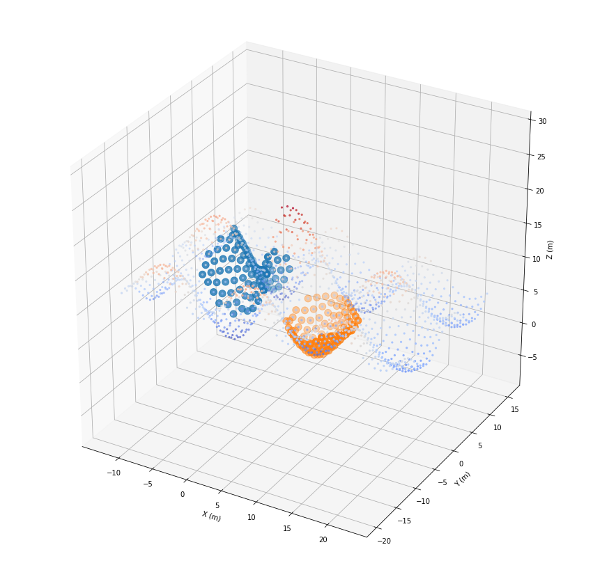
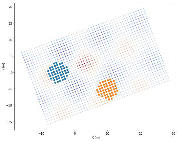
Radial filtering
We begin with filtering the points within a sphere around some points. As a result, we receive a list of point indices which can be used for sub-sampling.
[20]:
coords = [[-5, 0, 8], [10, -5, 5]]
r = 6.0
Once in 3D …
[21]:
fids_list = geoRecords.indexKD().ball(coords, r)
print(len(fids_list))
print(fids_list[0])
print(fids_list[1])
2
[308, 309, 310, 311, 358, 359, 360, 361, 362, 363, 408, 409, 410, 411, 412, 413, 414, 415, 416, 417, 418, 459, 460, 461, 462, 463, 464, 465, 466, 467, 468, 509, 510, 511, 512, 513, 514, 515, 516, 517, 560, 561, 562, 563, 564, 565, 566, 567, 610, 611, 612, 613, 614, 615, 616, 660, 661, 662, 663, 664, 665, 666, 667, 709, 710, 711, 712, 713, 714, 715, 716, 717, 759, 760, 761, 762, 763, 764, 765, 766, 767, 768, 808, 809, 810, 811, 812, 813, 814, 815, 816, 817, 818, 858, 859, 860, 861, 862, 863, 908, 909, 910, 911]
[679, 680, 681, 728, 729, 730, 731, 732, 777, 778, 779, 780, 781, 782, 783, 826, 827, 828, 829, 830, 831, 832, 833, 834, 876, 877, 878, 879, 880, 881, 882, 883, 884, 885, 925, 926, 927, 928, 929, 930, 931, 932, 933, 934, 935, 936, 975, 976, 977, 978, 979, 980, 981, 982, 983, 984, 985, 986, 1025, 1026, 1027, 1028, 1029, 1030, 1031, 1032, 1033, 1034, 1035, 1036, 1075, 1076, 1077, 1078, 1079, 1080, 1081, 1082, 1083, 1084, 1085, 1086, 1126, 1127, 1128, 1129, 1130, 1131, 1132, 1133, 1134, 1135, 1177, 1178, 1179, 1180, 1181, 1182, 1183, 1184, 1228, 1229, 1230, 1231, 1232, 1233]
[22]:
fig = plt.figure(figsize=(15, 15))
ax = plt.axes(projection='3d')
ax.set_xlim(axes_lims[0], axes_lims[3])
ax.set_ylim(axes_lims[1], axes_lims[4])
ax.set_zlim(axes_lims[2], axes_lims[5])
ax.set_xlabel('X (m)')
ax.set_ylabel('Y (m)')
ax.set_zlabel('Z (m)')

ax.scatter(*geoRecords.coords.T, c=geoRecords.z, cmap='coolwarm', marker='.')
for fids in fids_list:
    ax.scatter(*geoRecords[fids].coords.T, s=100)
plt.show()
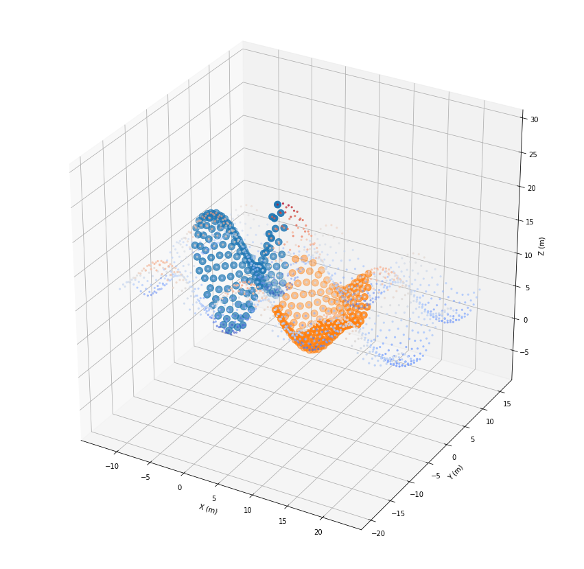
… and once in 2D.
[23]:
fids_list = geoRecords.indexKD(2).ball(coords, r)
[24]:
fig = plt.figure(figsize=(15, 15))
ax = plt.axes(projection='3d')
ax.set_xlim(axes_lims[0], axes_lims[3])
ax.set_ylim(axes_lims[1], axes_lims[4])
ax.set_zlim(axes_lims[2], axes_lims[5])
ax.set_xlabel('X (m)')
ax.set_ylabel('Y (m)')
ax.set_zlabel('Z (m)')

ax.scatter(*geoRecords.coords.T, c=geoRecords.z, cmap='coolwarm', marker='.')
for fids in fids_list:
    ax.scatter(*geoRecords[fids].coords.T, s=100)
plt.show()
Of course, we can do the same with the raster.
[25]:
fids_list = grid.indexKD().ball(coords, r)
[26]:
fig = plt.figure(figsize=(10, 10))
ax = plt.axes(aspect='equal')
plt.xlabel('X (m)')
plt.ylabel('Y (m)')

plt.scatter(*grid.records().coords.T, c=grid.records().z, cmap='coolwarm', marker='.')
for fids in fids_list:
    ax.scatter(*grid.records()[fids].coords.T)
plt.show()
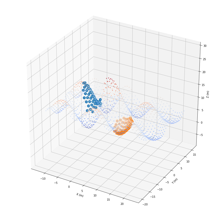
Nearest neighbor filtering
We can also filter the nearest neighbors of the points given before. Next to a list of point indices, we receive a list of point distances of the same shape.
[27]:
k=50
Once in 3D …
[28]:
dists_list, fids_list = geoRecords.indexKD().knn(coords, k)
[29]:
fig = plt.figure(figsize=(15, 15))
ax = plt.axes(projection='3d')
ax.set_xlim(axes_lims[0], axes_lims[3])
ax.set_ylim(axes_lims[1], axes_lims[4])
ax.set_zlim(axes_lims[2], axes_lims[5])
ax.set_xlabel('X (m)')
ax.set_ylabel('Y (m)')
ax.set_zlabel('Z (m)')

ax.scatter(*geoRecords.coords.T, c=geoRecords.z, cmap='coolwarm', marker='.')
for fids in fids_list:
    ax.scatter(*geoRecords[fids].coords.T, s=100)
plt.show()
… and once in 2D.
[30]:
dists_list, fids_list = geoRecords.indexKD(2).knn(coords, k)
[31]:
fig = plt.figure(figsize=(15, 15))
ax = plt.axes(projection='3d')
ax.set_xlim(axes_lims[0], axes_lims[3])
ax.set_ylim(axes_lims[1], axes_lims[4])
ax.set_zlim(axes_lims[2], axes_lims[5])
ax.set_xlabel('X (m)')
ax.set_ylabel('Y (m)')
ax.set_zlabel('Z (m)')

ax.scatter(*geoRecords.coords.T, c=geoRecords.z, cmap='coolwarm', marker='.')
for fids in fids_list:
    ax.scatter(*geoRecords[fids].coords.T, s=100)
plt.show()
And again, once with the raster.
[32]:
dists_list, fids_list = grid.indexKD(2).knn(coords, k)
[33]:
fig = plt.figure(figsize=(10, 10))
ax = plt.axes(aspect='equal')
plt.xlabel('X (m)')
plt.ylabel('Y (m)')

ax.scatter(*grid.records().coords.T, c=geoRecords.z, cmap='coolwarm', marker='.')
for fids in fids_list:
    ax.scatter(*grid.records()[fids].coords.T)
plt.show()
Point counting
We have the option to count the number of points within a given radius. For this purpose we select a subset of the raster first. Then, using the point cloud, we count the number of raster cells within the given radius.
[34]:
grid_subset = grid[15:25, 30:40]
count = grid_subset.indexKD(2).ball_count(r, geoRecords.coords)
print(count)
[0 0 0 ... 0 0 0]
[35]:
fig = plt.figure(figsize=(15, 15))
ax = plt.axes(projection='3d')
ax.set_xlim(axes_lims[0], axes_lims[3])
ax.set_ylim(axes_lims[1], axes_lims[4])
ax.set_zlim(axes_lims[2], axes_lims[5])
ax.set_xlabel('X (m)')
ax.set_ylabel('Y (m)')
ax.set_zlabel('Z (m)')

ax.scatter(*geoRecords.coords.T, c=count, cmap='YlOrRd')
ax.scatter(*grid_subset.records().coords.T, color='black')
ax.scatter(*grid.records().coords.T, color='gray', marker='.')
plt.show()
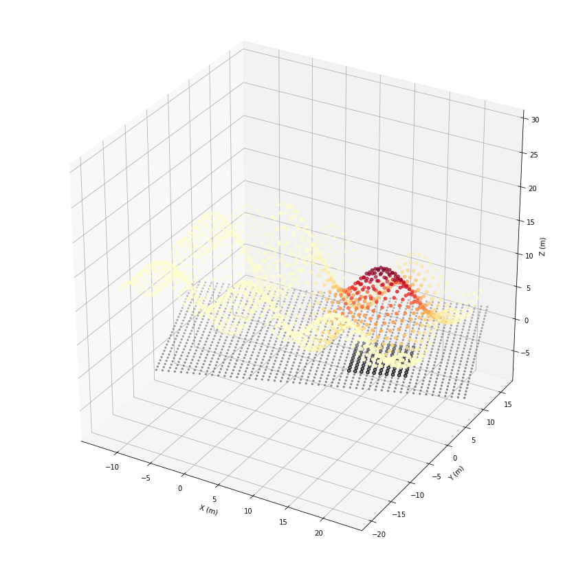
You might have noticed, that this was a fist step of data fusion, since we related the raster cells to the point cloud. This can also be done for nearest neighbor or similar spatial queries regardless of dimension.
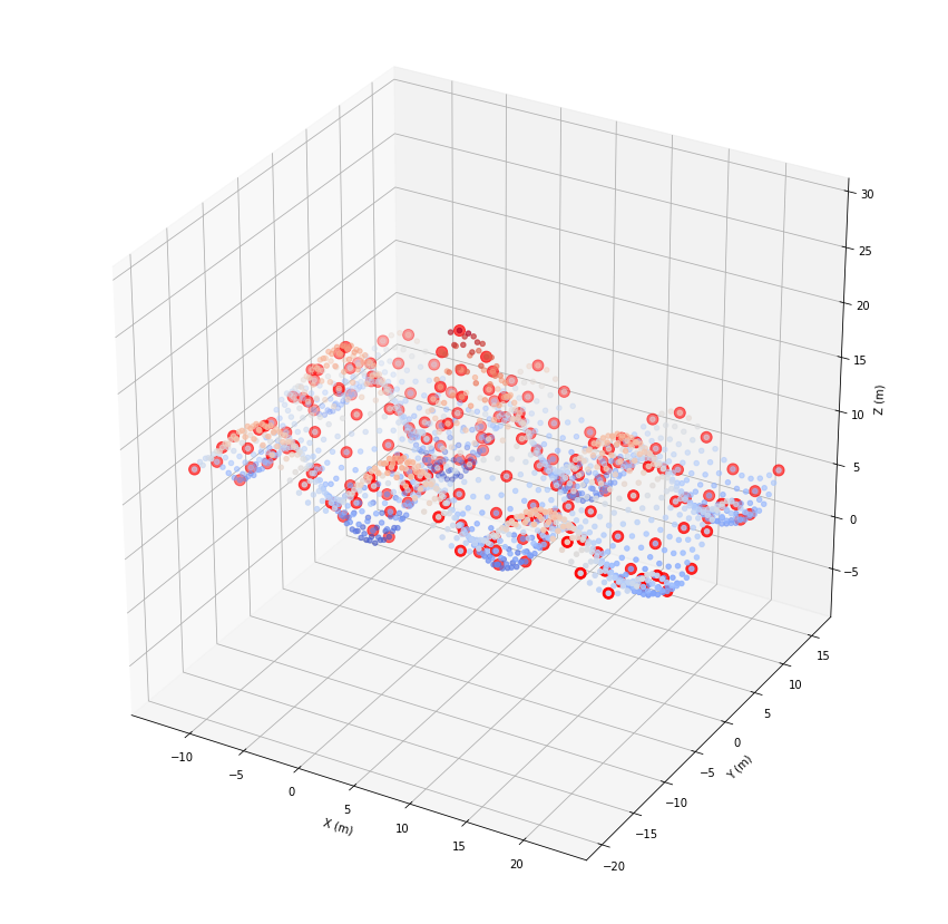
Point filters
To create a subset of points, we typically use some kind of point filters. We begin with a duplicate point filter. To ease the integration of such filters into your own algorithms, an iterator is returned instead of a list of point indices.
[36]:
fids = list(filters.ball(geoRecords.indexKD(), 2.5))
print(fids)
print(len(fids))
[620, 623, 618, 607, 472, 772, 519, 719, 625, 1372, 638, 1357, 505, 705, 1438, 610, 1474, 1470, 421, 821, 458, 758, 635, 617, 1404, 1274, 1459, 488, 788, 1288, 1270, 1255, 22, 603, 1435, 641, 475, 775, 7, 1441, 1259, 38, 405, 805, 627, 1172, 1285, 1468, 485, 785, 460, 760, 633, 1352, 1291, 612, 1427, 4, 791, 491, 25, 649, 468, 768, 1276, 1449, 616, 502, 702, 874, 374, 35, 19, 1483, 122, 1268, 1412, 107, 1107, 41, 1493, 1138, 307, 907, 10, 1203, 1261, 338, 938, 321, 921, 644, 1299, 1124, 629, 499, 799, 1332, 187, 1415, 1450, 477, 777, 1344, 532, 732, 885, 385, 1120, 1496, 1480, 49, 205, 1005, 1278, 1135, 546, 746, 353, 853, 274, 974, 125, 513, 713, 1141, 240, 170, 860, 360, 1250, 1266, 941, 443, 159, 1059, 1, 17, 450, 750, 44, 12, 1247, 32, 28, 844, 319, 919, 1126, 480, 780, 349, 949, 466, 766, 383, 883, 1102, 1231, 1194, 184, 1213, 97, 1118, 1034, 377, 877, 152, 395, 193, 952, 1098, 993, 226, 350, 311, 911, 66, 80, 946, 247, 1128, 112, 867, 367, 218, 1050, 880, 380, 414, 814, 1032, 232, 1116, 1062, 228, 1029, 166, 213, 966]
200
[37]:
fig = plt.figure(figsize=(15, 15))
ax = plt.axes(projection='3d')
ax.set_xlim(axes_lims[0], axes_lims[3])
ax.set_ylim(axes_lims[1], axes_lims[4])
ax.set_zlim(axes_lims[2], axes_lims[5])
ax.set_xlabel('X (m)')
ax.set_ylabel('Y (m)')
ax.set_zlabel('Z (m)')

ax.scatter(*geoRecords.coords.T, c=geoRecords.z, cmap='coolwarm')
ax.scatter(*geoRecords[fids].coords.T, color='red', s=100)
plt.show()
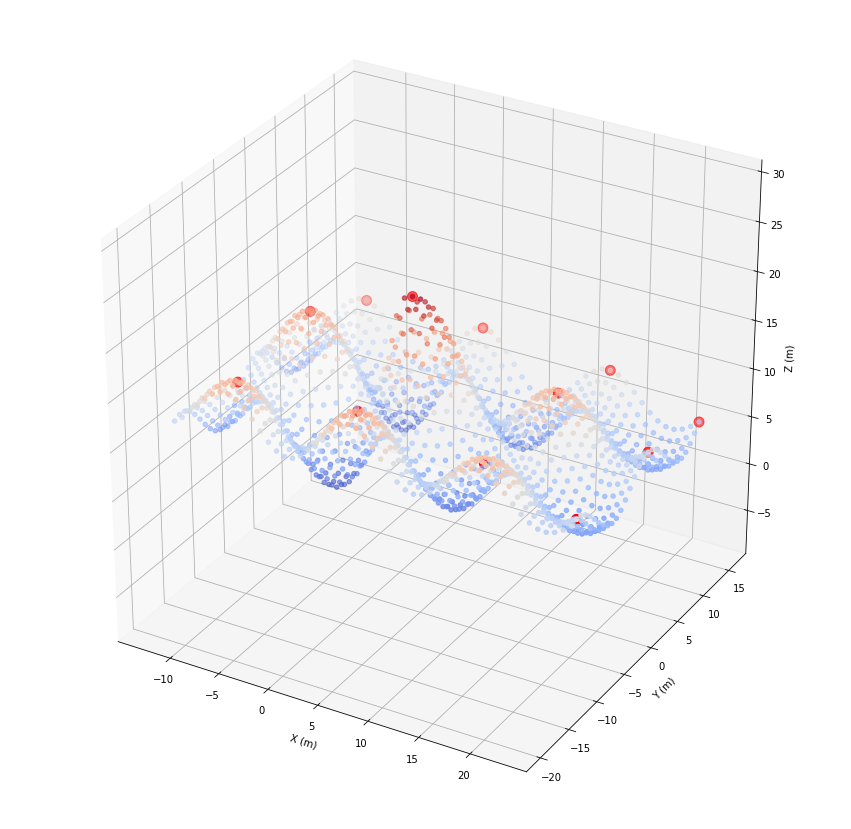
Sometimes we like to filter local maxima of an attribute using a given radius …
[38]:
fids = list(filters.extrema(geoRecords.indexKD(2), geoRecords.z, 1.5))
print(fids)
[620, 607, 1372, 638, 1357, 1438, 22, 7, 38, 649, 1449, 49]
[39]:
fig = plt.figure(figsize=(15, 15))
ax = plt.axes(projection='3d')
ax.set_xlim(axes_lims[0], axes_lims[3])
ax.set_ylim(axes_lims[1], axes_lims[4])
ax.set_zlim(axes_lims[2], axes_lims[5])
ax.set_xlabel('X (m)')
ax.set_ylabel('Y (m)')
ax.set_zlabel('Z (m)')

ax.scatter(*geoRecords.coords.T, c=geoRecords.z, cmap='coolwarm')
ax.scatter(*geoRecords[fids].coords.T, color='red', s=100)
plt.show()
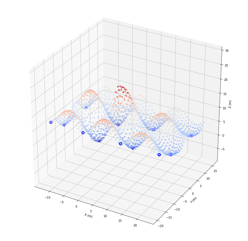
… or find local minima.
[40]:
fids = list(filters.extrema(geoRecords.indexKD(2), geoRecords.z, 1.5, inverse=True))
print(fids)
[265, 965, 1030, 230, 200, 1000, 246, 1046, 1464, 1480, 1496, 1450]
[41]:
fig = plt.figure(figsize=(15, 15))
ax = plt.axes(projection='3d')
ax.set_xlim(axes_lims[0], axes_lims[3])
ax.set_ylim(axes_lims[1], axes_lims[4])
ax.set_zlim(axes_lims[2], axes_lims[5])
ax.set_xlabel('X (m)')
ax.set_ylabel('Y (m)')
ax.set_zlabel('Z (m)')

ax.scatter(*geoRecords.coords.T, c=geoRecords.z, cmap='coolwarm')
ax.scatter(*geoRecords[fids].coords.T, color='blue', s=100)
plt.show()
Smoothing
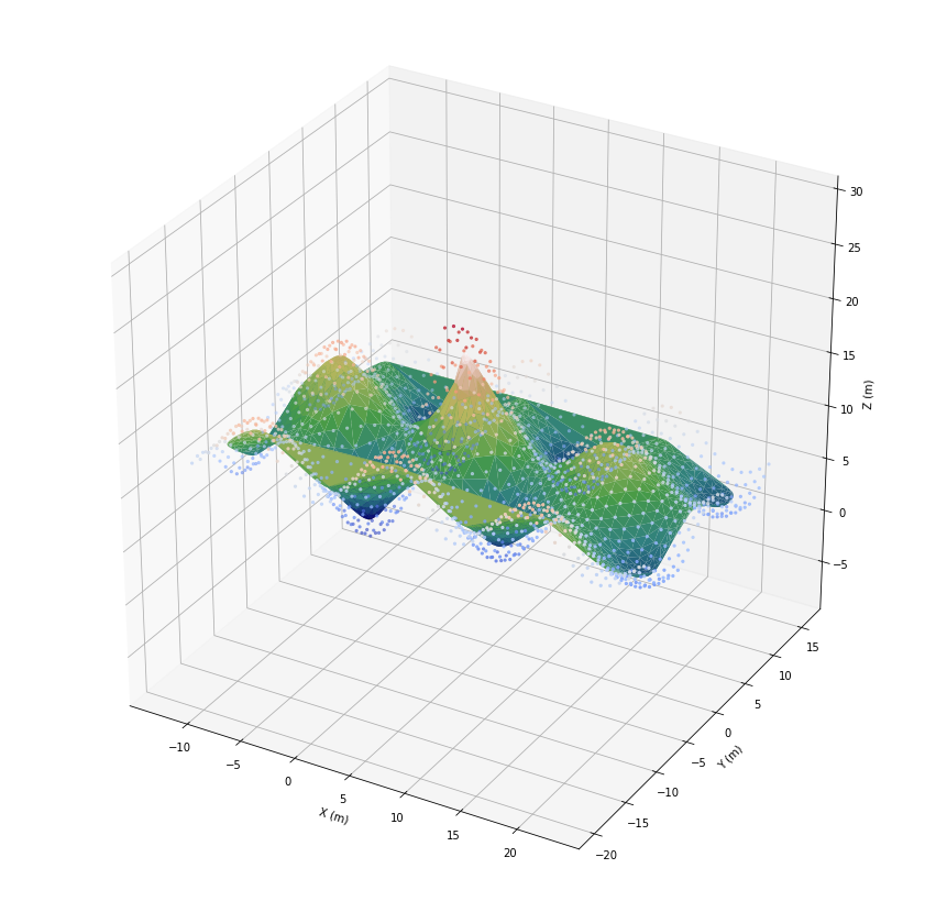
To compensate for noise, or receive just a smoother result we can use smoothing algorithms. The algorithm presented here averages the coordinates of the nearest neighbors.
[42]:
scoords = smoothing.mean_knn(geoRecords.coords, 20, num_iter=3)
[43]:
fig = plt.figure(figsize=(15, 15))
ax = plt.axes(projection='3d')
ax.set_xlim(axes_lims[0], axes_lims[3])
ax.set_ylim(axes_lims[1], axes_lims[4])
ax.set_zlim(axes_lims[2], axes_lims[5])
ax.set_xlabel('X (m)')
ax.set_ylabel('Y (m)')
ax.set_zlabel('Z (m)')

ax.scatter(*geoRecords.coords.T, c=geoRecords.z, cmap='coolwarm', marker='.')
ax.plot_trisurf(*scoords.T, cmap='gist_earth')
plt.show()
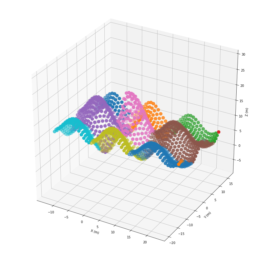
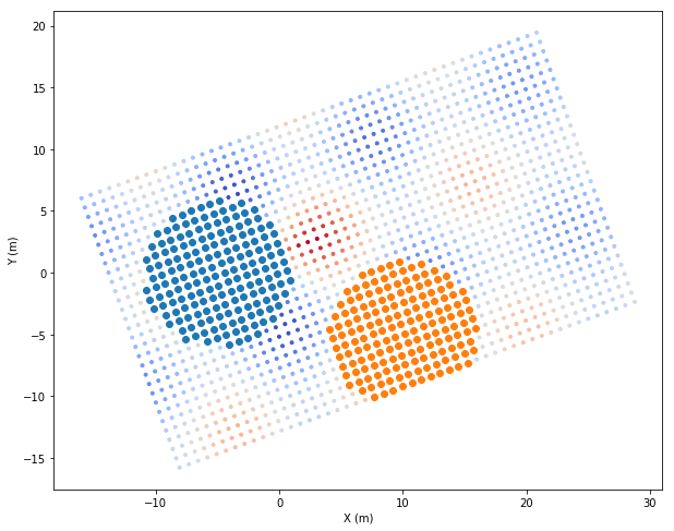
Clustering
A common problem is to cluster point clouds. Here we use a clustering algorithm, which assigns points iteratively to the most dominant class within a given radius. By iterating from top to bottom, the points are assigned to the hills of the surface.
[44]:
order = np.argsort(geoRecords.z)[::-1]
cluster_indices = clustering.majority_clusters(geoRecords.indexKD(), 5.0, order=order)
print(cluster_indices)
cluster_dict = classification.classes_to_dict(cluster_indices)
print(cluster_dict)
[ 7  7  7 ...  5  5 10]
{7: [0, 1, 2, 3, 4, 5, 6, 7, 8, 9, 10, 11, 12, 13, 50, 51, 52, 53, 54, 55, 56, 57, 58, 59, 60, 61, 62, 63, 101, 102, 103, 104, 105, 106, 107, 108, 109, 110, 111, 112, 154, 155, 156, 157, 158, 159, 160, 161], 6: [15, 16, 17, 18, 19, 20, 21, 22, 23, 24, 25, 26, 27, 28, 29, 64, 65, 66, 67, 68, 69, 70, 71, 72, 73, 74, 75, 76, 77, 78, 79, 80, 114, 115, 116, 117, 118, 119, 120, 121, 122, 123, 124, 125, 126, 127, 128, 129, 130, 165, 166, 167, 168, 169, 170, 171, 172, 173, 174, 175, 176, 177, 178, 179, 180, 217, 218, 219, 220, 221, 222, 223, 224, 225, 226, 227, 228, 229, 267, 268, 269, 270, 275, 276, 277, 278, 317, 318, 319, 327, 328], 8: [30, 31, 32, 33, 34, 35, 36, 37, 38, 39, 40, 41, 42, 43, 44, 45, 46, 47, 48, 81, 82, 83, 84, 85, 86, 87, 88, 89, 90, 91, 92, 93, 94, 95, 96, 97, 98, 99, 132, 133, 134, 135, 136, 137, 138, 139, 140, 141, 142, 143, 144, 145, 146, 147, 148, 149, 183, 184, 185, 186, 187, 188, 189, 190, 191, 192, 193, 194, 195, 196, 197, 198, 199, 234, 237, 238, 240, 241, 242, 243], 11: [49], 1: [100, 150, 151, 152, 162, 163, 164, 200, 201, 202, 203, 204, 206, 207, 208, 209, 210, 211, 212, 213, 214, 215, 216, 250, 251, 252, 253, 254, 255, 256, 257, 258, 259, 260, 261, 262, 263, 264, 265, 266, 300, 301, 302, 303, 304, 305, 306, 307, 308, 309, 310, 311, 312, 313, 314, 315, 316, 350, 351, 352, 353, 354, 355, 356, 357, 358, 359, 360, 361, 362, 363, 364, 365, 366, 367, 400, 401, 402, 403, 404, 405, 406, 407, 408, 409, 410, 411, 412, 413, 414, 415, 416, 417, 450, 451, 452, 453, 454, 455, 456, 457, 458, 459, 460, 461, 462, 463, 464, 465, 466, 500, 501, 502, 503, 504, 505, 506, 507, 508, 509, 510, 511, 512, 513, 514, 515, 550, 551, 552, 553, 554, 555, 556, 557, 558, 559, 560, 561, 562, 563, 564, 565, 600, 601, 602, 603, 604, 605, 606, 607, 608, 609, 610, 611, 612, 613, 614, 615, 650, 651, 652, 653, 654, 655, 656, 657, 658, 659, 660, 661, 662, 663, 664, 665, 700, 701, 702, 703, 704, 705, 706, 707, 708, 709, 710, 711, 712, 713, 714, 715, 750, 751, 752, 753, 754, 755, 756, 757, 758, 759, 760, 761, 762, 763, 764, 765, 766, 800, 801, 802, 803, 804, 805, 806, 807, 808, 809, 810, 811, 812, 813, 814, 815, 816, 817, 850, 851, 852, 853, 854, 855, 856, 857, 858, 859, 860, 861, 862, 863, 864, 865, 866, 867, 900, 901, 902, 903, 904, 905, 906, 907, 908, 909, 910, 911, 912, 913, 914, 915, 916, 952, 953, 954, 955, 956, 957, 958, 959, 960, 961, 962, 963, 964, 965, 1013, 1014, 1015], 3: [182, 231, 232, 233, 244, 245, 246, 247, 248, 249, 280, 281, 282, 283, 284, 285, 286, 287, 288, 289, 290, 291, 292, 293, 294, 295, 296, 297, 298, 299, 329, 330, 331, 332, 333, 334, 335, 336, 337, 338, 339, 340, 341, 342, 343, 344, 345, 346, 347, 348, 349, 379, 380, 381, 382, 383, 384, 385, 386, 387, 388, 389, 390, 391, 392, 393, 394, 395, 396, 397, 398, 399, 429, 430, 431, 432, 433, 434, 435, 436, 437, 438, 439, 440, 441, 442, 443, 444, 445, 446, 447, 448, 449, 480, 481, 482, 483, 484, 485, 486, 487, 488, 489, 490, 491, 492, 493, 494, 495, 496, 497, 498, 499, 530, 531, 532, 533, 534, 535, 536, 537, 538, 539, 540, 541, 542, 543, 544, 545, 546, 547, 548, 580, 581, 582, 583, 584, 585, 586, 587, 588, 589, 590, 591, 592, 593, 594, 595, 596, 597, 598, 631, 632, 633, 634, 635, 636, 637, 638, 639, 640, 641, 642, 643, 644, 645, 646, 647, 648, 680, 681, 682, 683, 684, 685, 686, 687, 688, 689, 690, 691, 692, 693, 694, 695, 696, 697, 698, 730, 731, 732, 733, 734, 735, 736, 737, 738, 739, 740, 741, 742, 743, 744, 745, 746, 747, 748, 780, 781, 782, 783, 784, 785, 786, 787, 788, 789, 790, 791, 792, 793, 794, 795, 796, 797, 798, 799, 829, 830, 831, 832, 833, 834, 835, 836, 837, 838, 839, 840, 841, 842, 843, 844, 845, 846, 847, 848, 849, 879, 880, 881, 882, 883, 884, 885, 886, 887, 888, 889, 890, 891, 892, 893, 894, 895, 896, 897, 898, 899, 930, 931, 932, 933, 934, 935, 936, 937, 938, 939, 940, 941, 942, 943, 944, 945, 946, 947, 948, 949, 981, 982, 983, 984, 985, 986, 987, 988, 989, 990, 991, 992, 993, 994, 996, 997, 998, 999], 0: [272, 273, 320, 321, 322, 323, 324, 325, 326, 368, 369, 370, 371, 372, 373, 374, 375, 376, 377, 418, 419, 420, 421, 422, 423, 424, 425, 426, 427, 428, 467, 468, 469, 470, 471, 472, 473, 474, 475, 476, 477, 478, 479, 517, 518, 519, 520, 521, 522, 523, 524, 525, 526, 527, 528, 529, 566, 567, 568, 569, 570, 571, 572, 573, 574, 575, 576, 577, 578, 579, 616, 617, 618, 619, 620, 621, 622, 623, 624, 625, 626, 627, 628, 629, 630, 666, 667, 668, 669, 670, 671, 672, 673, 674, 675, 676, 677, 678, 679, 717, 718, 719, 720, 721, 722, 723, 724, 725, 726, 727, 728, 729, 767, 768, 769, 770, 771, 772, 773, 774, 775, 776, 777, 778, 779, 818, 819, 820, 821, 822, 823, 824, 825, 826, 827, 828, 868, 869, 870, 871, 872, 873, 874, 875, 876, 877, 920, 921, 922, 923, 924, 925, 926, 972, 973], 9: [549, 599, 649, 699, 749], 2: [917, 918, 919, 927, 928, 929, 966, 967, 968, 969, 970, 975, 976, 977, 978, 979, 980, 1016, 1017, 1018, 1019, 1020, 1021, 1022, 1023, 1024, 1025, 1026, 1027, 1028, 1029, 1030, 1031, 1064, 1065, 1066, 1067, 1068, 1069, 1070, 1071, 1072, 1073, 1074, 1075, 1076, 1077, 1078, 1079, 1080, 1115, 1116, 1117, 1118, 1119, 1120, 1121, 1122, 1123, 1124, 1125, 1126, 1127, 1128, 1129, 1130, 1165, 1166, 1167, 1168, 1169, 1170, 1171, 1172, 1173, 1174, 1175, 1176, 1177, 1178, 1179, 1215, 1216, 1217, 1218, 1219, 1220, 1221, 1222, 1223, 1224, 1225, 1226, 1227, 1228, 1229, 1265, 1266, 1267, 1268, 1269, 1270, 1271, 1272, 1273, 1274, 1275, 1276, 1277, 1278, 1279, 1315, 1316, 1317, 1318, 1319, 1320, 1321, 1322, 1323, 1324, 1325, 1326, 1327, 1328, 1329, 1365, 1366, 1367, 1368, 1369, 1370, 1371, 1372, 1373, 1374, 1375, 1376, 1377, 1378, 1379, 1415, 1416, 1417, 1418, 1419, 1420, 1421, 1422, 1423, 1424, 1425, 1426, 1427, 1428, 1429, 1465, 1466, 1467, 1468, 1469, 1470, 1471, 1472, 1473, 1474, 1475, 1476, 1477, 1478, 1479], 4: [950, 951, 1000, 1001, 1002, 1003, 1004, 1005, 1007, 1008, 1009, 1010, 1011, 1012, 1050, 1051, 1052, 1053, 1054, 1055, 1056, 1057, 1058, 1059, 1060, 1061, 1062, 1063, 1100, 1101, 1102, 1103, 1104, 1105, 1106, 1107, 1108, 1109, 1110, 1111, 1112, 1113, 1114, 1150, 1151, 1152, 1153, 1154, 1155, 1156, 1157, 1158, 1159, 1160, 1161, 1162, 1163, 1164, 1200, 1201, 1202, 1203, 1204, 1205, 1206, 1207, 1208, 1209, 1210, 1211, 1212, 1213, 1214, 1250, 1251, 1252, 1253, 1254, 1255, 1256, 1257, 1258, 1259, 1260, 1261, 1262, 1263, 1264, 1300, 1301, 1302, 1303, 1304, 1305, 1306, 1307, 1308, 1309, 1310, 1311, 1312, 1313, 1314, 1350, 1351, 1352, 1353, 1354, 1355, 1356, 1357, 1358, 1359, 1360, 1361, 1362, 1363, 1364, 1400, 1401, 1402, 1403, 1404, 1405, 1406, 1407, 1408, 1409, 1410, 1411, 1412, 1413, 1414, 1450, 1451, 1452, 1453, 1454, 1455, 1456, 1457, 1458, 1459, 1460, 1461, 1462, 1463, 1464], 5: [1032, 1033, 1034, 1035, 1036, 1037, 1038, 1039, 1040, 1041, 1042, 1043, 1044, 1045, 1046, 1047, 1048, 1049, 1081, 1082, 1083, 1084, 1085, 1086, 1087, 1088, 1089, 1090, 1091, 1092, 1093, 1094, 1095, 1096, 1097, 1098, 1099, 1131, 1132, 1133, 1134, 1135, 1136, 1137, 1138, 1139, 1140, 1141, 1142, 1143, 1144, 1145, 1146, 1147, 1148, 1149, 1180, 1181, 1182, 1183, 1184, 1185, 1186, 1187, 1188, 1189, 1190, 1191, 1192, 1193, 1194, 1195, 1196, 1197, 1198, 1199, 1230, 1231, 1232, 1233, 1234, 1235, 1236, 1237, 1238, 1239, 1240, 1241, 1242, 1243, 1244, 1245, 1246, 1247, 1248, 1249, 1280, 1281, 1282, 1283, 1284, 1285, 1286, 1287, 1288, 1289, 1290, 1291, 1292, 1293, 1294, 1295, 1296, 1297, 1298, 1299, 1330, 1331, 1332, 1333, 1334, 1335, 1336, 1337, 1338, 1339, 1340, 1341, 1342, 1343, 1344, 1345, 1346, 1347, 1348, 1380, 1381, 1382, 1383, 1384, 1385, 1386, 1387, 1388, 1389, 1390, 1391, 1392, 1393, 1394, 1395, 1396, 1397, 1398, 1430, 1431, 1432, 1433, 1434, 1435, 1436, 1437, 1438, 1439, 1440, 1441, 1442, 1443, 1444, 1445, 1446, 1447, 1448, 1480, 1481, 1482, 1483, 1484, 1485, 1486, 1487, 1488, 1489, 1490, 1491, 1492, 1493, 1494, 1495, 1496, 1497, 1498], 10: [1349, 1399, 1449, 1499]}
[45]:
fig = plt.figure(figsize=(15, 15))
ax = plt.axes(projection='3d')
ax.set_xlim(axes_lims[0], axes_lims[3])
ax.set_ylim(axes_lims[1], axes_lims[4])
ax.set_zlim(axes_lims[2], axes_lims[5])
ax.set_xlabel('X (m)')
ax.set_ylabel('Y (m)')
ax.set_zlabel('Z (m)')

for fids in cluster_dict.values():
    ax.scatter(*geoRecords[fids].coords.T, s=100)
plt.show()