ICP for point cloud alignment

In this tutorial we will learn to align several point clouds using two variants of the Iterative Closest Point (ICP) [1] algorithm.

We begin with loading the required modules.

import numpy as np

from pyoints import (
    storage,
    Extent,
    transformation,
    filters,
    registration,
    normals,
)

from mpl_toolkits import mplot3d
import matplotlib.pyplot as plt
from matplotlib import animation
from IPython.display import HTML

%matplotlib inline

Preparing the data

We load three point clouds of the Standfort Bunny [2] dataset. The original PLY files have been converted to a binary format to spare disc space and speed up loading time.

A = storage.loadPly('bun000_binary.ply')
print(A.shape)
print(A.dtype.descr)

(40256,)
[('coords', '<f4', (3,))]

B = storage.loadPly('bun045_binary.ply')
print(B.shape)
print(B.dtype.descr)

(40097,)
[('coords', '<f4', (3,))]

C = storage.loadPly('bun090_binary.ply')
print(C.shape)
print(C.dtype.descr)

(30379,)
[('coords', '<f4', (3,))]

We filter the point cloud to receive sparse point clouds more suitable for visualization. Thinning the point clouds also speeds up the ICP algorithm.

r = 0.004
A = A[list(filters.ball(A.indexKD(), r))]
B = B[list(filters.ball(B.indexKD(), r))]
C = C[list(filters.ball(C.indexKD(), r))]

Before we visualize the point cloud, we define the colors and axes limits.

axes_lims = Extent([
    A.extent().center - 0.5 * A.extent().ranges.max(),
    A.extent().center + 0.5 * A.extent().ranges.max()
])
colors = {'A': 'green', 'B': 'blue', 'C': 'red'}

fig = plt.figure(figsize=(15, 15))
ax = plt.axes(projection='3d')
ax.set_xlim(axes_lims[0], axes_lims[3])
ax.set_ylim(axes_lims[1], axes_lims[4])
ax.set_zlim(axes_lims[2], axes_lims[5])
ax.set_xlabel('X (m)')
ax.set_ylabel('Y (m)')
ax.set_zlabel('Z (m)')

ax.scatter(*A.coords.T, color=colors['A'])
ax.scatter(*B.coords.T, color=colors['B'])
ax.scatter(*C.coords.T, color=colors['C'])
plt.show()

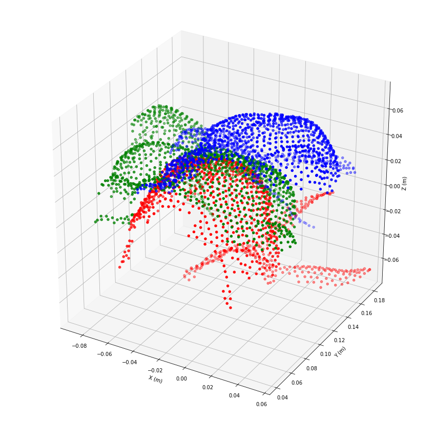
We can see, that the point clouds B and C are rotated by 45 and 90 degree. Since the ICP algorithm assumes already roughly aligned point clouds as an input, we rotate the point clouds accordingly. But, to harden the problem a bit, we use slightly differing rotation angles.

T_A = transformation.r_matrix([90*np.pi/180, 0, 0])
A.transform(T_A)
T_B = transformation.r_matrix([86*np.pi/180, 0, 45*np.pi/180])
B.transform(T_B)
T_C = transformation.r_matrix([95*np.pi/180, 0, 90*np.pi/180])
C.transform(T_C)

rec.array([([ 0.06625563, -0.01275   ,  0.05892337],),
           ([ 0.06583019, -0.0105    ,  0.05548104],),
           ([ 0.06577063, -0.01575   ,  0.05616905],), ...,
           ([-0.06031808, -0.05075   ,  0.1382622 ],),
           ([-0.06160365, -0.054     ,  0.12657075],),
           ([-0.06041196, -0.0495    ,  0.14218831],)],
          dtype=[('coords', '<f4', (3,))])

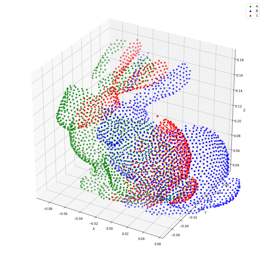
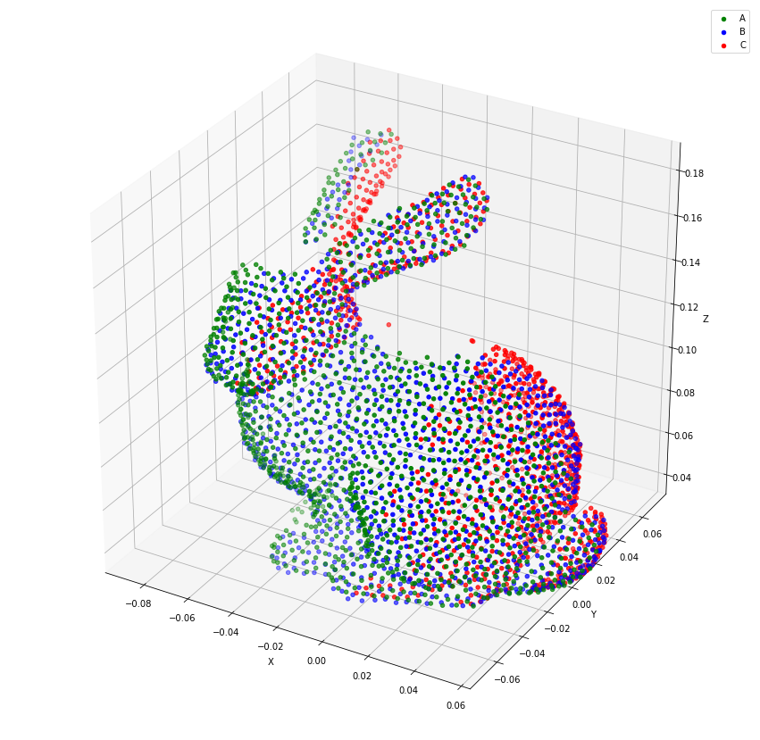
We update axes limits and visualize the point clouds again. The resulting point clouds serve as input for the ICP algorithm.

axes_lims = Extent([
    A.extent().center - 0.5 * A.extent().ranges.max(),
    A.extent().center + 0.5 * A.extent().ranges.max()
])

fig = plt.figure(figsize=(15, 15))
ax = plt.axes(projection='3d')
ax.set_xlim(axes_lims[0], axes_lims[3])
ax.set_ylim(axes_lims[1], axes_lims[4])
ax.set_zlim(axes_lims[2], axes_lims[5])
ax.set_xlabel('X')
ax.set_ylabel('Y')
ax.set_zlabel('Z')

ax.scatter(*A.coords.T, color=colors['A'], label='A')
ax.scatter(*B.coords.T, color=colors['B'], label='B')
ax.scatter(*C.coords.T, color=colors['C'], label='C')
ax.legend()
plt.show()

ICP algorithm

We begin with preparing the input data. Our ICP implementation expects a dictionary of point sets as an input.

coords_dict = {
    'A': A.coords,
    'B': B.coords,
    'C': C.coords
}

First, we initialize an ICP object. The algorithm iteratively matches the ‘k’ closest points. To limit the ratio of mismatched points, the ‘radii’ parameter is provided. It defines an ellipsoid within points can be assigned.

d_th = 0.04
radii = [d_th, d_th, d_th]
icp = registration.ICP(
    radii,
    max_iter=60,
    max_change_ratio=0.000001,
    k=1
)

After initialization, we apply the ICP algorithm to our dataset. The algorithm returns three dictionaries. The first dictionary provides the final roto-translation matrices of the point clouds. The second specifies the corresponding point matches. The third dictionary gives some information on the convergence of the algorithm.

T_dict, pairs_dict, report = icp(coords_dict)

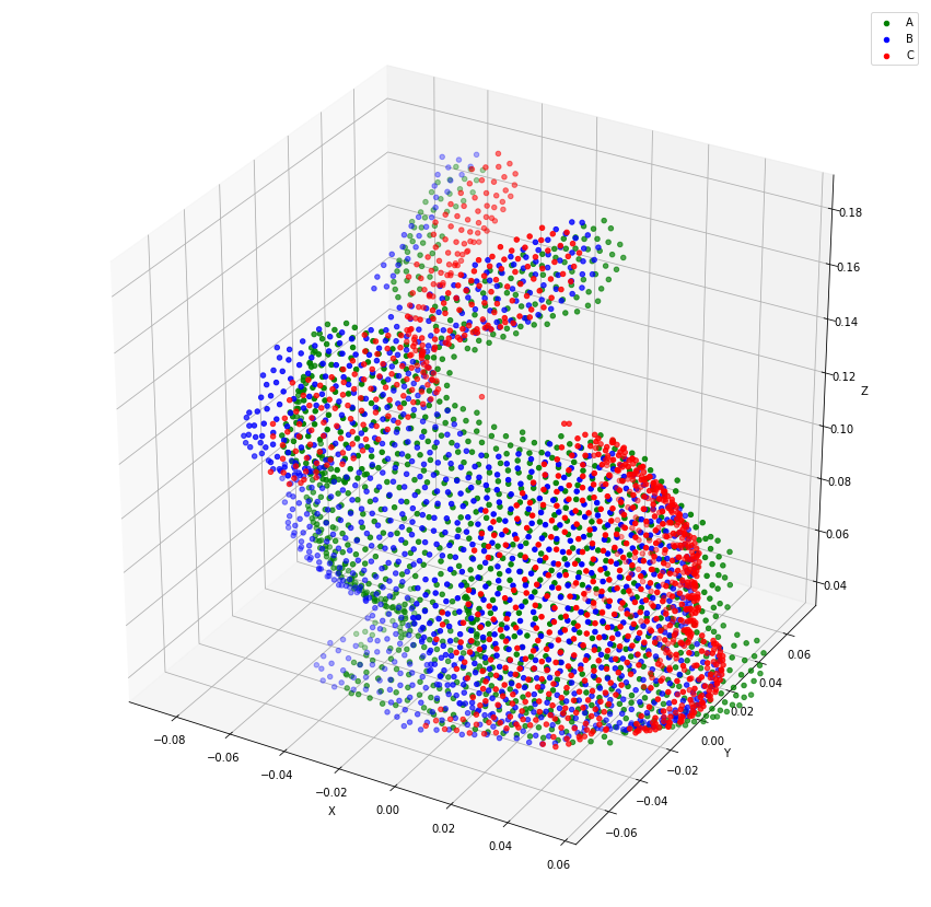
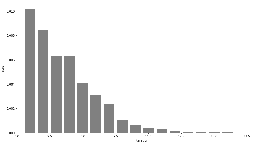
Let’s visualize the resulting point sets and the Root Mean Squared Error (RMSE).

fig = plt.figure(figsize=(15, 15))
ax = plt.axes(projection='3d')
ax.set_xlim(axes_lims[0], axes_lims[3])
ax.set_ylim(axes_lims[1], axes_lims[4])
ax.set_zlim(axes_lims[2], axes_lims[5])
ax.set_xlabel('X')
ax.set_ylabel('Y')
ax.set_zlabel('Z')

for key in coords_dict:
    coords = transformation.transform(coords_dict[key], T_dict[key])
    ax.scatter(*coords.T, color=colors[key], label=key)
ax.legend()
plt.show()

fig = plt.figure(figsize=(15, 8))
plt.xlim(0, len(report['RMSE']) + 1)
plt.xlabel('Iteration')
plt.ylabel('RMSE')

plt.bar(np.arange(len(report['RMSE']))+1, report['RMSE'], color='gray')
plt.show()

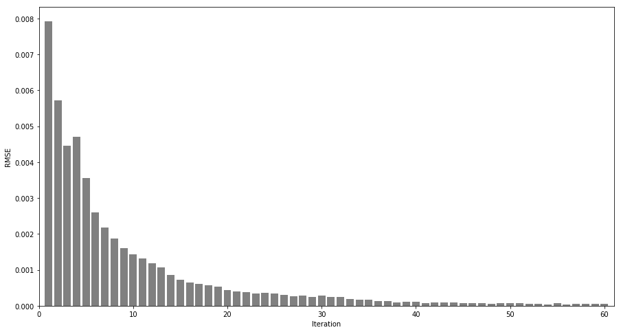
Although the result is not perfect, the point clouds have been aligned. The remaining misalignment is most likely caused by a lot of mismatched points.

NICP algorithm

Inspired by the idea of a Normal ICP algorithm proposed by Serafin and Grisetti [3] [4], a ICP variant has been developed which considers the surface orientation of the points.

We begin with calculating and displaying the surface normals.

normals_dict = {
    key: normals.fit_normals(coords_dict[key], k=5, preferred=[0, -1, 0])
    for key in coords_dict
}

fig = plt.figure(figsize=(15, 15))
ax = plt.axes(projection='3d')
ax.set_xlim(axes_lims[0], axes_lims[3])
ax.set_ylim(axes_lims[1], axes_lims[4])
ax.set_zlim(axes_lims[2], axes_lims[5])
ax.set_xlabel('X')
ax.set_ylabel('Y')
ax.set_zlabel('Z')

ax.scatter(*A.coords.T, c=normals_dict['A'][:, 2], cmap='coolwarm')
for coord, normal in zip(coords_dict['A'], normals_dict['A']):
    ax.plot(*np.vstack([coord, coord + normal*0.01]).T, color='black')
plt.show()

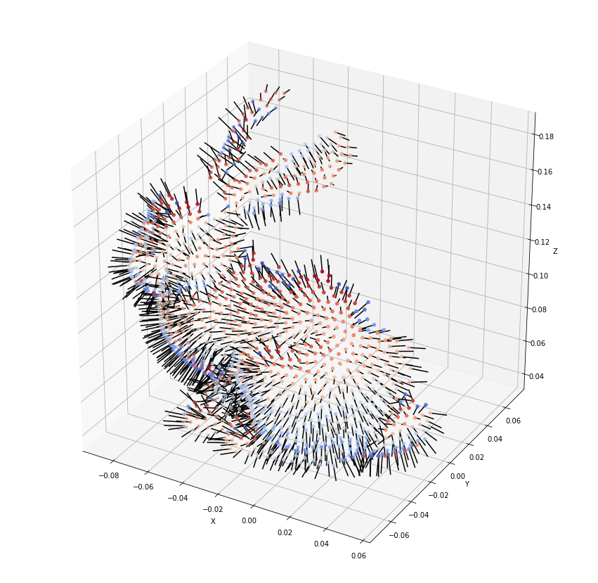
The surface orientation should reduce the ratio of mismatched points. Now, we create the NICP instance. A six dimensional ellipsoid is defined which takes into account the point distances, as well as the normal differences.

n_th = np.sin(15 * np.pi / 180)
radii = [d_th, d_th, d_th, n_th, n_th, n_th]
nicp = registration.ICP(
    radii,
    max_iter=60,
    max_change_ratio=0.000001,
    update_normals=True,
    k=1
)

The NICP instance is used to apply the algorithm.

T_dict, pairs_dict, report = nicp(coords_dict, normals_dict)

fig = plt.figure(figsize=(15, 15))
ax = plt.axes(projection='3d')
ax.set_xlim(axes_lims[0], axes_lims[3])
ax.set_ylim(axes_lims[1], axes_lims[4])
ax.set_zlim(axes_lims[2], axes_lims[5])
ax.set_xlabel('X')
ax.set_ylabel('Y')
ax.set_zlabel('Z')

for key in coords_dict:
    coords = transformation.transform(coords_dict[key], T_dict[key])
    ax.scatter(*coords.T, color=colors[key], label=key)
ax.legend()
plt.show()

fig = plt.figure(figsize=(15, 8))
plt.xlim(0, len(report['RMSE']) + 1)
plt.xlabel('Iteration')
plt.ylabel('RMSE')

plt.bar(np.arange(len(report['RMSE']))+1, report['RMSE'], color='gray')
plt.show()

We can see, that the convergence rate of the NICP algorithm is much better compared to the traditional ICP algorithm. In particular, the alignment is more plausible.

Finally, we create an animation to visualize the convergence.

fig = plt.figure(figsize=(8, 8))
ax = plt.axes(projection='3d')
ax.set_xlim(axes_lims[0], axes_lims[3])
ax.set_ylim(axes_lims[1], axes_lims[4])
ax.set_zlim(axes_lims[2], axes_lims[5])
fig.tight_layout()

# initializing plot
artists={
    key: ax.plot([],[],[], '.', color=colors[key], label=key)[0]
    for key in coords_dict
}
ax.legend()

# collecting the roto-translation matrices
T_iter = [{key: np.eye(4) for key in coords_dict}] + report['T']

def animate(i):
    # updates the frame
    ax.set_xlabel('Iteration %i' % i)
    for key in coords_dict:
            coords = transformation.transform(coords_dict[key], T_iter[i][key])
            artists[key].set_data(coords[:, 0], coords[:, 1])
            artists[key].set_3d_properties(coords[:, 2])
    return artists.values()

# creates the animation
anim = animation.FuncAnimation(fig, animate, frames=range(len(T_iter)), interval=250, blit=True)

# save as GIF
anim.save('nicp.gif', writer=animation.ImageMagickWriter())
plt.close()
# display as HTML (online version only)
HTML(anim.to_jshtml())

Once Loop Reflect

References

[1] P.J. Besl and N.D. McKay (1992): ‘A Method for Registration of 3-D Shapes’, IEEE Transactions on Pattern Analysis and Machine Intelligence, vol. 14 (2): 239-256.

[2] Stanford University Computer Graphics Laboratory, (1993): ‘Stanford Bunny’, URL https://graphics.stanford.edu/data/3Dscanrep/ (accessed January 17, 2019).

[3] J. Serafin and G. Grisetti (2014): ‘Using augmented measurements to improve the convergence of icp’, International Conference on Simulation, Modeling, and Programming for Autonomous Robots. Springer, Cham: 566-577.

[4] J. Serafin and G. Grisetti (2014): ‘NICP: Dense normal based pointcloud registration’, International Conference on Intelligent Robots and Systems (IROS): 742-749.